This is the final post in a series about non-destructively inspecting chips with the IRIS (Infra-Red, in-situ) technique. Here are links to previous posts:

• IRIS project overview
• Methodology
• Light source electronics
• Fine focus stage
• Light source mechanisms
• Machine control & focus software

This post will cover the software used to stitch together smaller images generated by the control software into a single large image. My IRIS machine with a 10x objective generates single images that correspond to a patch of silicon that is only 0.8mm wide. Most chips are much larger than that, so I take a series of overlapping images that must be stitched together to generate a composite image corresponding to a full chip.

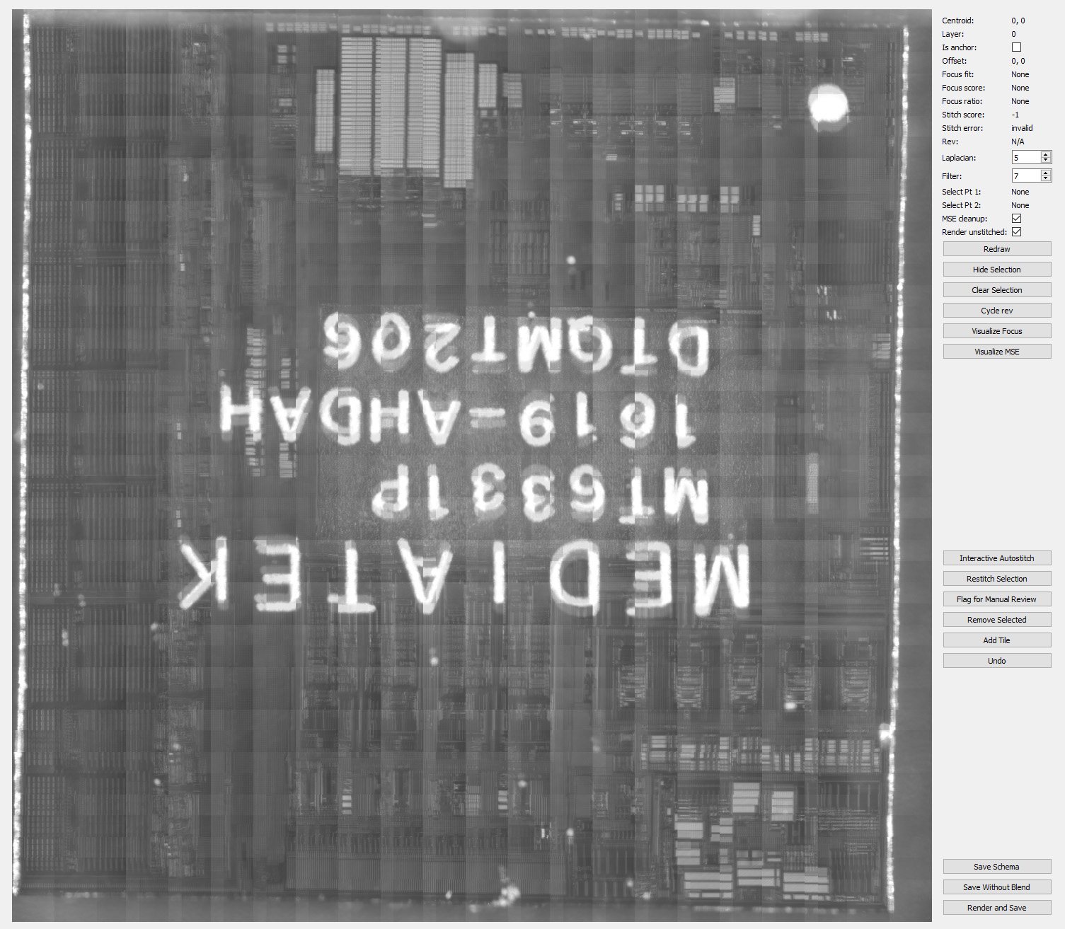
The un-aligned image tiles look like this:

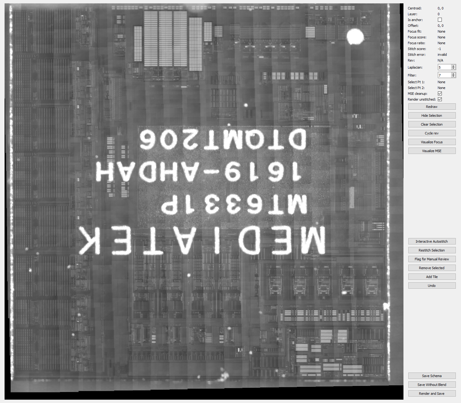
And the stitching software assembles it into something like this:

The problem we have to solve is that even though we command the microscope to move to regularly spaced intervals, in reality, there is always some error in the positioning of the microscope. The accuracy is on the order of 10’s of microns at best, but we are interested in extracting features much smaller than that. Thus, we must rely on some computational methods to remove these error offsets.

At first one might think, “this is easy, just throw it into any number of image stitching programs used to generate panoramas!”. I thought that too.

However, it turns out these programs perform poorly on images of chips. The most significant challenge is that chip features tend to be large, repetitive arrays. Most panorama algorithms rely on a step of “feature extraction” where it uses some algorithms to decide what’s an “interesting” feature and line them up between two images. These algorithms are tuned for aesthetically pleasing results on images of natural subjects, like humans or outdoor scenery; they get pretty lost trying to make heads or tails out of the geometrically regular patterns in a chip image. Furthermore, the alignment accuracy requirement for an image panorama is not as strict as what we need for IRIS. Most panaroma stitchers rely on a later pass of seam-blending to iron out deviations of a few pixels, yielding aesthetic results despite the misalignments.

Unfortunately, we’re looking to post-process these images with an image classifier to perform a gate count census, and so we need pixel-accurate alignment wherever possible. On the other hand, because all of the images are taken by machine, we never have to worry about rotational or scale adjustments – we are only interested in correcting translational errors.

Thus, I ended up rolling my own stitching algorithm. This was yet another one of those projects that started out as a test program to check data quality, and suffered from “just one more feature”-itis until it blossomed into the heaping pile that it is today. I wouldn’t be surprised if there were already good quality chip stitching programs out there, but, I did need a few bespoke features and it was interesting enough to learn how to do this, so I ended up writing it from scratch.

Well, to be accurate, I copy/pasted lots of stackoverflow answers, LLM-generated snippets, and boilerplate from previous projects together with heaps of glue code, which I think qualifies as “writing original code” these days? Maybe the more accurate way to state it is, “I didn’t fork another program as a starting point”. I started with an actual empty text buffer before I started copy-pasting five-to-twenty line code snippets into it.

Sizing Up the Task

A modestly sized chip of a couple dozen square millimeters generates a dataset of a few hundred images, each around 2.8MiB in size, for a total dataset of a couple gigabytes. While not outright daunting, it’s enough data that I can’t be reckless, yet small enough that I can get away with lazy decisions, such as using the native filesystem as my database format.

It turns out that for my application, the native file system is a performant, inter-operable, multi-threaded, transparently memory caching database format. Also super-easy to make backups and to browse the records. As a slight optimization, I generate thumbnails of every image on the first run of the stitching program to accelerate later drawing operations for preview images.

Each file’s name is coded with its theoretical absolute position on the chip, along with metadata describing the focus and lighting parameters, so each file has a name something like this:

x0.00_y0.30_z10.00_p6869_i3966_t127_j4096_u127_a0.0_r1_f8.5_s13374_v0.998_d1.5_o100.0.png

It’s basically an underscore separated list of metadata, where each element is tagged with a single ASCII character, followed by its value. It’s a little awkward, but functional and easy enough to migrate as I upgrade schemas.

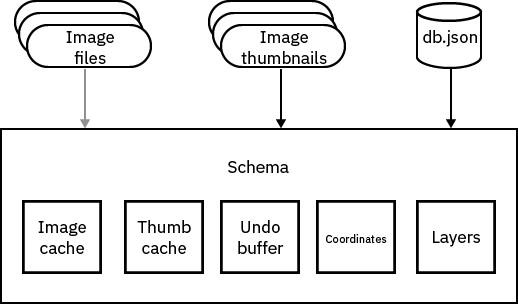
Creating a Schema

All of the filenames are collated into a single Python object that tracks the transformations we do on the data, as well as maintains a running log of all the operations (allowing us to have an undo buffer). I call this the “Schema” object. I wish I knew about dataframes before I started this project, because I ended up re-implementing a lot of dataframe features in the course of building the Schema. Oh well.

The Schema object is serialized into a JSON file called “db.json” that allows us to restore the state of the program even in the case of an unclean shutdown (and there are plenty of those!).

The initial state of the program is to show a preview of all the images in their current positions, along with a set of buttons that control the state of the stitcher, select what regions to stitch/restitch, debugging tools, and file save operations. The UI framework is a mix of PyQt and OpenCV’s native UI functions (which afaik wrap PyQt objects).

Above: screenshot of the stitching UI in its initial state.

At startup, all of the thumbnails are read into memory, but none of the large images. There’s an option to cache the images in RAM as they are pulled in for processing. Generally, I’ve had no trouble just pulling all the images into RAM because the datasets haven’t exceeded 10GiB, but I suppose once I start stitching really huge images, I may need to do something different.

…Or maybe I just buy a bigger computer? Is that cheating? Extra stick of RAM is the hundred-dollar problem solver! Until it isn’t, I suppose. But, the good news is there’s a strong upper bound of how big of an image we’d stitch (e.g. chips rarely go larger than the reticle size) and it’s probably around 100GiB, which somehow seems “reasonable” for an amount of RAM to put in one desktop machine these days.

Again, my mind boggles, because I spend most of my time writing Rust code for a device with 16MiB of RAM.

Auto Stitching Flow

At the highest level, the stitching strategy uses a progressive stitch, starting from the top left tile and doing a “lawn mower” pattern. Every tile looks “left and up” for alignment candidates, so the very top left tile is considered to be the anchor tile. This pattern matches the order in which the images were taken, so the relative error between adjacent tiles is minimized.

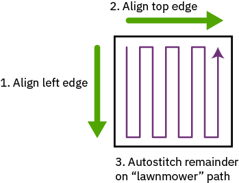
Before lawn mowing, a manually-guided stitch pass is done along the left and top edges of the chip. This usually takes a few minutes, where the algorithm runs in “single step” mode and the user reviews and approves of each alignment individually. The reason this is done is if there are any stitching errors on the top or left edge, it will propagate throughout the process, so these edges must be 100% correct before the algorithm can run unattended. It is also the case that the edges of a chip can be quite tricky to stitch, because arrays of bond pads can look identical across multiple frames, and accurate alignment ends up relying upon random image artifacts caused by roughness in the die’s physical edges.

Once the left and top edges are fixed, the algorithm can start in earnest. For each tile, it starts with a “guess” of where the new tile should go based on the nominal commanded values of the microscope. It then looks “up” and “left” and picks the tile that has the largest overlapping region for the next step.

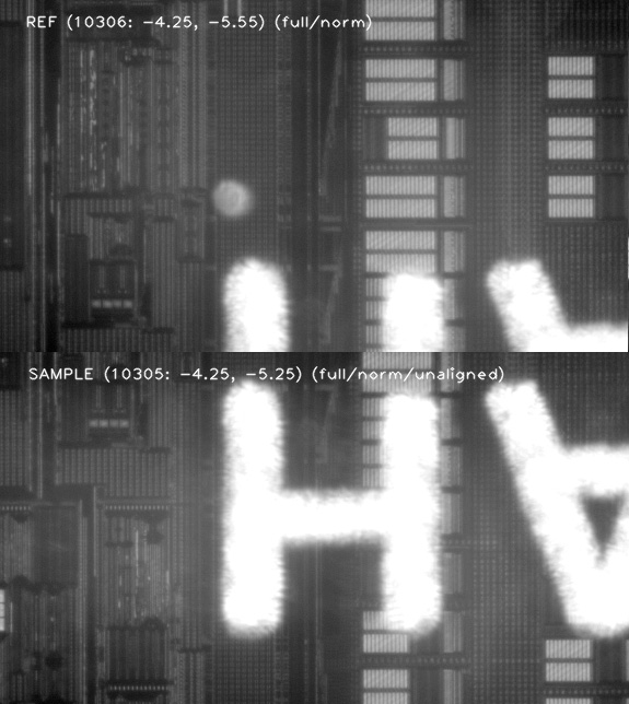
Above is an example of the algorithm picking a tile in the “up” direction as the “REF” (reference) tile with which to stitch the incoming tile (referred to as “SAMPLE”). The image above juxtaposes both tiles with no attempt to align them, but you can already see how the top of the lower image partially overlaps with the bottom of the upper image.

Template Matching

Next, the algorithm picks a “template” to do template matching. Template matching is an effective way to align two images that are already in the same orientation and scale. The basic idea is to pick a “unique” feature in one image, and convolve it with every point in the other image. The point with the highest convolution value is probably going to be the spot where the two images line up.

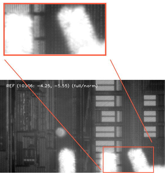
Above: an example of a template region automatically chosen for searching across the incoming sample for alignment.

In reality, the algorithm is slightly more complicated than this, because the quality of the match greatly depends on the quality of the template. Thus we first have to answer the question of what template to use, before we get to where the template matches. This is especially true on chips, because there are often large, repeated regions that are impossible to uniquely match, and there is no general rule that can guarantee where a unique feature might end up within a frame.

Thus, the actual implementation also searches for the “best” template using brute-force: it divides the nominally overlapping region into potential template candidates, and computes the template match score for all of them, and picks the template that produces the best alignment of all the candidates. This is perhaps the most computationally intensive step in the whole stitching process, because we can have dozens of potential template candidates, each of which must be convolved over many of the points in the reference image. Computed sequentially on my desktop computer, the search can take several seconds per tile to find the optimal template. However, Python makes it pretty easy to spawn threads, so I spawn one thread per candidate template and let them duke it out for CPU time and cache space. Fortunately I have a Ryzen 7900X, so with 12 cores and 12MiB of L2 cache, the entire problem basically fits entirely inside the CPU, and the multi-threaded search completes in a blink of the eye.

This is another one of those moments where I feel kind of ridiculous writing code like this, but somehow, it’s a reasonable thing to do today.

The other “small asterisk” on the whole process is that it works not on the original image, but it works on a Gaussian-filtered, Laplacian-transformed version of the images. In other words, instead of matching against the continuous tones of an image, I do the template match against the edges of the image, making the algorithm less sensitive to artifacts such as lens flare, or global brightness gradients.

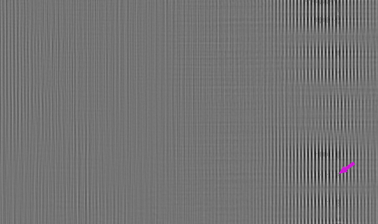
Above is an example of the output of the template matching algorithm. Most of the region is gray, which indicates a poor match. Towards the right, you start to see “ripples” that correspond to the matching features starting to line up. As part of the algorithm, I extract contours to ring regions with a high match, and pick the center of the largest matching region, highlighted here with the pink arrow. The whole contour extraction and center picking thing is a native library in OpenCV with pretty good documentation examples.

Minimum Squared Error (MSE) Cleanup

Template matching usually gets me a solution that aligns images to within a couple of pixels, but I need every pixel I can get out of the alignment, especially if my plan is to do a gate count census on features that are just a few pixels across. So, after template alignment, I do a “cleanup” pass using a minimum squared error (MSE) method.

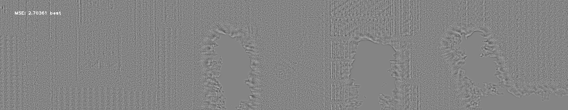
Above: example of the MSE debugging output. This illustrates a “good match”, because most of the image is gray, indicating a small MSE. A poor match would have more image contrast.

MSE basically takes every pixel in the reference image and subtracts it from the sample image, squares it, and sums all of them together. If the two images were identical and exactly aligned, the error would be zero, but because the images are taken with a real camera that has noise, we can only go as low as the noise floor. The cleanup pass starts with the initial alignment proposed by the template matching, and computes the MSE of the current alignment, along with candidates for the image shifted one pixel up, left, right and down. If any of the shifted candidates have a lower error, the algorithm picks that as the new alignment, and repeats until it finds an alignment where the center pixel has the lowest MSE. To speed things up, the MSE is actually done at two levels of shifting, first with a coarse search consisting of several pixels, and finally with a fine-grained search at a single pixel level. There is also a heuristic to terminate the search after too many steps, because the algorithm is subject to limit cycles.

Because each step of the search depends upon results from the previous step, it doesn’t parallelize as well, and so sometimes the MSE search can take longer than the multi-threaded template matching search, especially when the template search really blew it and we end up having to search over a dozens of pixels to find the true alignment (but if the template matching did it’s job, the MSE cleanup pass is barely noticeable).

Again, the MSE search works on the Gaussian-filtered Laplacian view of the image, i.e., it’s looking at edges, not whole tones.

After template matching and MSE cleanup, the final alignment goes through some basic sanity checks, and if all looks good, moves on to the next tile. If something doesn’t look right – for example, the proposed offsets for the images are much larger than usual, or the template matcher found too many good solutions (as is the case on stitching together very regular arrays like RAM) – the algorithm stops and the user can manually select a new template and/or move the images around to find the best MSE fit. This will usually happen a couple of times per chip, but can be more frequent if there were focusing problems or the chip has many large, regular arrays of components.

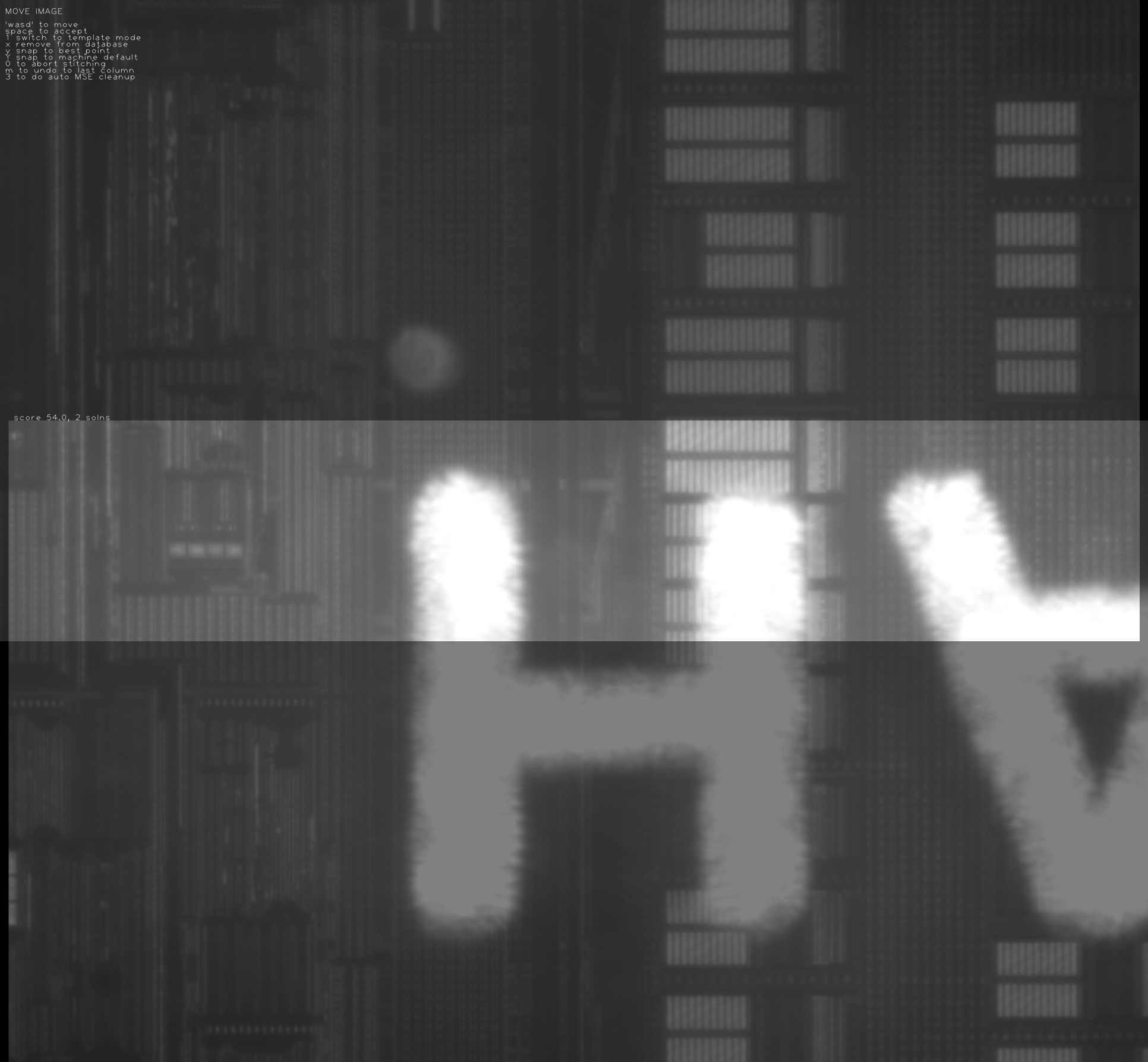
Above: the automatically proposed stitching alignment of the two images in this example. The bright area is the overlapping region between the two adjacent tiles. Note how there is a slight left-right offset that the algorithm detected and compensated for.

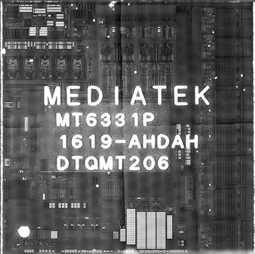
Once the stitching is all finished, you end up with a result that looks a bit like this:

Here, all the image tiles are properly aligned, and you can see how the Jubilee machine (Jubilee is the motion platform on which IRIS was built) has a slight “walk off” as evidenced by the diagonal pattern across the bottom of the preview area.

Potential Hardware Improvements

The Jubilee uses a CoreXY belt path, which optimizes for minimum flying mass. The original designers of the Jubilee platform wanted it to perform well in 3D printing applications, where print speed is limited by how fast the tool can move. However, any mismatch in belt tension leads to the sort of “walk off” visible here. I basically need to re-tension the machine every couple of weeks to minimize this effect, but I’m told that this isn’t typical. It’s possible that I might have defective belts or more likely, sloppy assembly technique; or I live in the tropics and the room has 60% relative humidity even with air conditioning, causing the belts to expand slightly over time as they absorb moisture. Or it could be that the mass of the microscope is pretty enormous, and that amplifies the effect of slight mismatches in tensioning.

Regardless of the root cause, the Jubilee’s design intent of performing well in 3D printing applications incurs some trade-off in terms of maintenance level required to sustain absolute accuracy. Since in the IRIS application, microscope head speed is not important, tool mass is already huge, and precision is paramount, one of the mods I’m considering for my version of the platform is redoing the belt layout so that the drive is Cartesian instead of CoreXY. That should help minimize the walk-off and reduce the amount of maintenance needed to keep it running in top-notch condition.

Edge Blending for Aesthetics

You’ll note that in the above image the overlap of the individual tiles is readily apparent, due to slight variations in brightness across the imaging field. This can probably be improved by adding some diffusers, and also improving the alignment of the lights relative to the focal point (it’s currently off by a couple of millimeters, because I designed it around the focal point of a 20x objective, but these images were taken with a 10x objective). Even then, I suspect some amount of tiling will always be visible, because the human eye is pretty sensitive to slight variations in shades of gray.

My working hypothesis is that the machine learning driven standard cell census (yet to be implemented!) will not care so much about the gradient because it only ever looks at regions a few dozen pixels across in one go. However, in order to generate a more aesthetically pleasing image for human consumption, I implemented a blending algorithm to smooth out the edges, which results in a final image more like this:

Click the image to browse a full resolution version, hosted on siliconpr0n.

There’s still four major stitch regions visible, and this is because OpenCV’s MultiBandBlender routine seems to be limited to handle 8GiB-ish of raw image data at once, so I can’t quite blend whole chips in a single go. I tried running the same code on a machine with a 24GiB graphics card, and got the same out of memory error, so the limit isn’t total GPU memory. When I dug in a bit, it seemed like there was some driver-level limitation related to the maximum number of pointers to image buffers that I was hitting, and I didn’t feel like shaving that yak.

The underlying algorithm used to do image blending is actually pretty neat, and based off a paper from 1983(!) by Burt and Adelson titled “A Multiresolution Spline with Application to Image Mosaics”. I actually tried implementing this directly using OpenCV’s Image Pyramid feature, mainly because I couldn’t find any documentation on the MultiBandBlender routine. It was actually pretty fun and insightful to play around with image pyramids; it’s a useful idiom for extracting image features at vastly different scales, and for all its utility it’s pretty memory efficient (the full image pyramid consumes about 1.5x of the original image’s memory).

However, it turns out that the 1983 paper doesn’t tell you how to deal with things like non power of 2 images, non-square images, or images that only partially overlap…and I couldn’t find any follow-up papers that goes into these “edge cases”. Since the blending is purely for aesthetic appeal to human eyes, I decided not to invest the effort to chase down these last details, and settled for the MultiBandBlender, stitch lines and all.

Touch-Ups

The autostitching algorithm isn’t perfect, so I also implemented an interface for doing touch-ups after the initial stitching pass is done. The interface allows me to do things like flag various tiles for manual review, automatically re-stitch regions, and visualize heat maps of MSE and focus shifts.

The above video is a whistlestop tour of the stitching and touch-up interface.

All of the code discussed in this blog post can be found in the iris-stitcher repo on github. stitch.py contains the entry point for the code.

That’s a Wrap!

That’s it for my blog series on IRIS, for now. As of today, the machine and associated software is capable of reliably extracting reference images of chips and assembling them into full-chip die shots. The next step is to train some CNN classifiers to automatically recognize logic cells and perform a census of the number of gates in a given region.

Someday, I also hope to figure out a way to place rigorous bounds on the amount of logic that could be required to pass an electrical scan chain test while also hiding malicious Hardware Trojans. Ideally, this would result in some sort of EDA tool that one can use to insert an IRIS-hardened scan chain into an existing HDL design. The resulting fusion of design methodology, non-destructive imaging, and in-circuit scan chain testing may ultimately give us a path towards confidence in the construction of our chips.

And as always, a big shout-out to NLnet and to my Github Sponsors for allowing me to do all this research while making it openly accessible for anyone to replicate and to use.

This entry was posted on Monday, April 22nd, 2024 at 6:56 pm and is filed under IRIS. You can follow any responses to this entry through the RSS 2.0 feed. You can leave a response, or trackback from your own site.